「BroWithAIInfra」纯种网安老头简单学学 CMU11868
其实自己已经学了很多次了,但是因为没做笔记,于是学完又忘了。
痛定思痛,重新开始吧,正好 CMU11868 26’Fall 的课程也差不多开始了(2026-08-24),不如直接重新来吧(笑
Before we start…
我们建立对应的文件夹,下载资源。
我使用 WebBridge 配合 Claude 将 Slides / Resources 下载下来(书本资源我从 zlib 下下来了 orz,好孩子别学),利用 MinerU 解析 PDF 获取 markdown + 图片。
这里 SKILL 没有做太多的干涉,一个写完之后问另外几个 agent 怎么改进,优化了一波。
Lecture 01 - Introduction to the LLMs
题外话,真先进啊,已经把 K3 放到图里了。
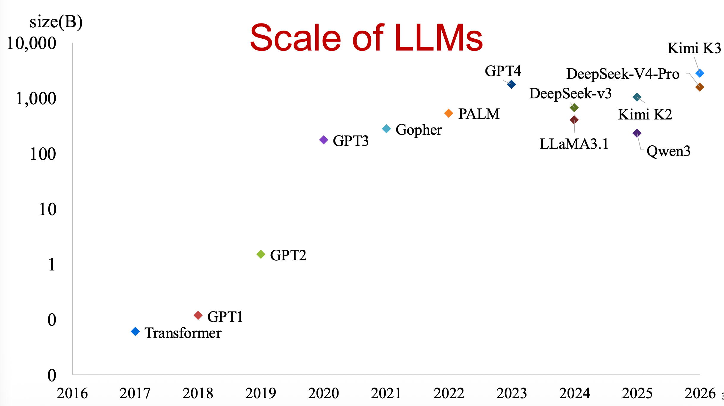
跳过那些讲 LLM 能力的东西,我们只需要知道,Modern LLM focus on:
- Generalist —— 通才,把所有任务都可以抽象成 token-based sequence generation。也是直接把像是 NLP 那边的翻译、分类、摘要之类的那套每个任务做一套不同的假设 / 抽象 / 优化全部干翻了。这也是 AI Infra 爽的原因,底层一优化下层应用全受益。
- Instructibility
- Agentic
Mathematical Foundations
所谓 LLM,本质上就是在做一件事:给定一段 prompt ,在产生序列 的前提下,求产生下一个 token 的概率,或者说就是给定一段前缀,输出词表上的概率分布。
把 next_token 泛化到整个回答,其实也就是这么一个东西:
举一个具体例子:
不难注意这个也就是为什么我们 decode 阶段只能串行,因为必须要知道前序才能算出这个链式的概率,当然其实在训练的时候,因为这个整句话已经是 ground truth 了,其实就可以直接并行去训,叫 Teacher Forcing
其实现在也有一些 so-called 并行的方案。例如 Speculative Decoding / MTP,但是其实都不是严格意义的并行。我们会在后面的内容里讲。
然后 LLM 一般就是分成三类,Encoder Only / Decoder Only / Encoder & Decoder
其实这里我一直觉得名字很神秘,Encoder 和 Decoder 很容易想成是密码学里面那种编解码的东西。硬要说的话 Encoder 就是编码一个词与其他词之间关系的这么一个东西吧!
Encoder-only
对于 Encoder Only,他们是*非自回归(Non-autoregressive, NAR)*的,以 BERT 为例,它实际上就是具体在这个 B(idirection) 上,它是能看到双向(前、后)信息的,通过掩码预测的方式训练。
这个好处一眼就能看出来,以翻译来说,所有的 都不依赖于 ,而都只依赖于 ,这也就说明我们可以直接并行去生成,速度显然好;
坏处也很明显,之前产生的东西没法看到,这种 条件独立 很容易带来 多峰问题(Multimodality Problem),除此之外,也事先需要长度信息。
举个最简单的例子:“翻译 teacher成中文“。
在这个任务上,假设训练集里面 “老师” 和 “先生” 分布平均。
第一个位置看,选了 “老”;第二个位置看,选了 “生”。
结果答案就变成了 “老生”。
P(y₁, y₂) ≠ P(y₁)P(y₂)
Encoder-Decoder
就是 ,encoder 那边把词和词之间关系学明白了。然后整组向量就丢给 decoder,decoder 想看哪个就直接看(也就是交叉注意力)。具体细节后面讲 transformer 的时候再写吧。
encoder-decoder 其实天然适配翻译的活,因为想要翻译,我们一定得看完整个句子,这个天然符合 encoder 的思想(虽然 decode-only 其实也能做到);同时,翻译更像是一个 bijection 的活,它是一一对应的,这点和摘要啊,问答之类的活还不一样,这就导致我们的交叉注意力其实在这个上面和它的数学形式是更加同构的;此外,翻译也是少有的不缺少配对语料的任务(但是可惜,架不住通用语料比他多了几个数量级,导致这种配对其实直接被学进去了)
Decoder-only
现在最流行的形式。之前说到了配对语料的缺失其实就是催生 Decoder-only 架构的最大原因,虽然它纯建模能力不如 Encoder-Decoder,但是得益于数据易得性 / 参数复用 / 推理状态简单等先天优势,所以还是被最广泛使用。
Training
一般来说我们都使用 交叉熵(Cross Entropy, CE) 损失来表示真实分布与模型分布的差距,或者我平常记它形式靠 负对数似然(NegativeLogLikelihood, NLL) —— 这俩在 One-Hot 这种语言标签下其实数学形式是完全一样的,在这种情况下,最小化交叉熵损失其实也就是 最大似然估计(Maximum Likelihood Estimate, MLE)。
不过其实差别还是挺大的,因为 CE 其实还有其他性质,而且在非 One-Hot 的情况下,两个就完全不一样了。CE 的数学形式可以写成下面的形式:
其中 代表词表, 代表真实分布, 代表模型分布。
至于为什么和 NLL 一致,是因为在语言模型下面,对于 ,只在它的真实位置有 ,而其他地方都是 ,因此最后也是:
当然,其实在 PyTorch 里,我们可以看到 nn.CrossEntropyLoss(logits, target) == nn.NLLLoss(log_softmax(logits), target)。所以其实在 PyTorch 里,CE 和 NLL 的区别就是 logits 到底传原始的还是 log_softmax 之后的而已。当然,在 Infra 层面,这里更是有其他的考量,例如,显存上的考量,我们在后续把一些概念解释后再仔细讲。
不过上面这么说其实容易误导,因为在 PPT 里,CE 其实写成这样:
不过仔细分析一下其实就可以发现,我们上面说的 CE 是 针对于一个 token,而这里的 CE 则是 针对于句子里的一个位置,写完整如下,但是就因为我们刚才说到的 One-Hot 的原因,所以就化简了。
那么如何衡量模型好坏呢?最简单也是 PPL(Perplexity),其实就是套个
这是啥意思呢?我们取一个随机模型,它的输出接近均匀分布,每个 token 的概率都是 。此时 ,所以 ;而对于真实分布,也容易算出它的数学下界 。所以我们可以简单这样理解:PPL 就是代表模型在 每一步 上在 多少个 等可能的候选之间摇摆。
以 GPT-3 在 Penn Treebank 上为例,它训练是 300B Tokens,而 zero shot 下,它的 PPL 大概是 20.5
当然除了 PPL,例如 pass@k 之类的也在不同的下游任务中进行测量。
Challenges
Slide 上就这么一句话。
Key system problem: compute (train/inference) larger LLMs on bigger datasets with fewer resources (GPU/memory/power) faster
也就是四个量:
整个 LLM 其实就是在这四个维度上做优化做 trade off,放到 low-level 上,我们可以把它们拆成 4 个原语
- MatMul 矩阵乘 ,唯一一个 compute-bound 的原语(相对来说)
- Reduct 归约
- Map 映射
- Memory Movement 内存移动
在 Data Movement is All You Need 里面提到,这些几乎不做运算的算子,其实占了接近 的运行时间。所以,算子优化的一大要点反而是如何减少 内存移动 的次数,而不只是如何减少 计算次数
当然,上面的思路其实是完全在 low-level 的情况下讨论的,实际上不同的层也有不同的关注要点,而总的效率往往是所有层的效率相乘算出来的。
例如,在集群里,我们考虑的可能更多就是 scheduling / scaling 之类的事情;而在框架层,我们可能更考虑 easy dev 。

slide 的图其实已经完全描述了整个优化任务,也对应后续课程的不同内容。当然,不只是 scale up,scale down 也是任务之一(量化、蒸馏、端侧部署都需要小模型)
Lecture 02
Updated at 2026-08-17
想要做优化,我们肯定得通过数学的方式定义整个目标。而其实严格意义上来说,算力这件事是我们本身无法操控的,所以其实上最后的优化还是落在了 算子的计算次数 以及 通信 上面。我们可以以一个 “平衡点” 来定义整个优化目标,也就是说,对于一个 的卡来说,每从 HBM 里取 1Byte 的数据,我们得至少做 次浮点计算,才能配得上这个卡的算力,否则,如果高于它,就是 compute-bound,低于它,则是 memory-bound,对应了不同的优化目标。
而整个课基本上都在不同层的数据传输带宽上做文章。
举一个例子,假设某个算子在 A100 上的算术强度是 I=200FLOP/Byte,A100 的内存带宽是 2.04TB/s,峰值算力是 312TF,平衡点是 153。问这个算子在 H100 上的情况(H100 内存带宽 3.35TB/s,峰值算力 989TF,平衡点 295)。
不难注意,这个算子在 A100 上属于 compute-bound 的情况,给了这么多字节但是算不完;而在 H100 上则是 memory-bound 的情况,没这么多字节给你算。它在 H100 上的实际算力就是 ,也就是 ,而 H100 的算力提升实际上却是 ,差了 。也就是说,我买一张 H100,其实上就用到了它 68% 的性能,也是算一次就亏一次钱。
那咋办呢,看这个公式,增加带宽可以做到,或者换一个词,增加通信效率。例如,算子融合 (kernel fusion),我们把多个算子放在一起做,让各种数据从寄存器里拿出来直接开算,省去了存中间结果以及拿中间结果的 HBM 通信开销,那么带宽也就美美增加了,这也是我们后面会说到的 FlashAttention 等的思路。
warp / block / etc…
感觉刚上手 GPU programming 的时候,应该最容易乱的就是这里。
首先我们应该区分出哪些是软件侧的实现和哪些是硬件侧的实现。
软件侧:
一个 Grid 相当于就是 GPU 本身,gridDim 就是一个 Grid 里有多少个 Block
一个 Block 就相当于是一个运行组,这个组里面的所有线程独占一个 SharedMemory
至于 Warp,它更像是软硬件的结合点。但是在写 kernel 的时候,还是要记得,虽然你写是以一个 thread 来写,但其实底层还是在调度一个 warp,做优化也应该从这一层来思考。
Grid ← 一次 kernel 启动的全部├── Block 0 ← 你指定有几个、每个多大│ ├── Warp 0 (thread 0-31) ← ⚠️ 你控制不了,硬件自动切│ ├── Warp 1 (thread 32-63)│ └── ...├── Block 1└── ...硬件侧:
硬件底层是以 SM 作为调度单元的。每个 SM 又有 4 个 Partition,一个 Partition 又有 32 条 Lane。
GPU (A6000)└── 84 × SM (Streaming Multiprocessor) └── 4 × Partition ← 每个有 1 个 warp scheduler └── 32 × Lane ← 就是所谓的 "CUDA core"聪明的你可能已经发现了,32 Lane,那不就和我们 Warp 有 32 个线程对上了吗?那一个 Partition 其实就是一个 Warp?太聪明了,你已经打通了软硬件的视角。这里的 32 Lane 其实就是每一个 Partition 会同时执行这 32 Lane 的同一条指令。而 4 Partition 自然也就代表每周期可以 issue 4 条不同的 warp 指令了。像这样向上分析,你也就能知道 SM 就是一个 Block 了。
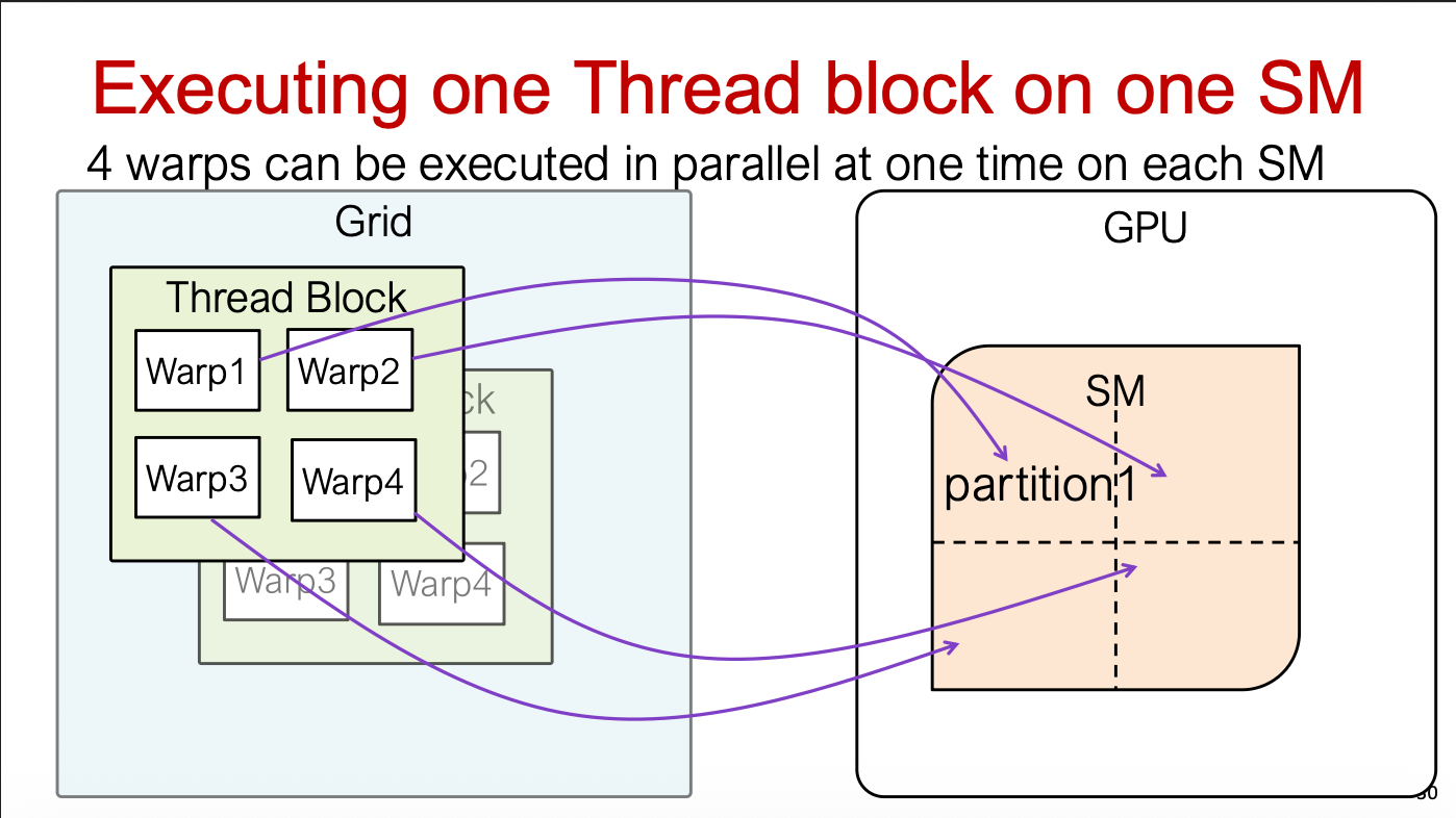
这么一思考,可能大概也许你就能把软硬件的视角打通了,做到写软件思考硬件,哈哈。
举一个🌰
__global__ void VecAddKernel(int* A, int* B, int* C, int n) { int i = blockDim.x * blockIdx.x + threadIdx.x; if (i < n) C[i] = A[i] + B[i];}// n = 1024VecAddKernel<<<4, 256>>>(dA, dB, dC, 1024);软件侧:
| 数量 | 来源 | |
|---|---|---|
| block | 4 | 代码定义,一般就 ceil(n / blockDim),例如这里就是 ceil(1024 / 256)=4 |
| 每 block 线程 | 256 | 代码定义,一般就固定 128 / 256 |
| 每 block warp | 8 | 256 / 32 |
| 总 warp | 32 | 4 × 8 |
| 总线程 | 1024 | 4 × 256 |
索引怎么算的 —— 以 block 2 的第 5 号线程为例:
它负责 C[517] = A[517] + B[517]。每个线程只干一个元素,全部 1024 个线程覆盖整个数组。
硬件侧:
- 4 个 block → 派到 4 个不同的 SM → 不难发现 84 个 SM 里 80 个全程闲置
- 每个 SM 上的 8 个 warp → 均分给该 SM 的 4 个 partition,每个 partition 2 个 warp
- 每个 warp 的 32 个线程 → 32 条 lane 同时执行同一条指令
聪明的你一定发现了几个问题:
-
如果 block 分少了,好像我的 SM 就闲置了啊。
没错,所以如果可能的话,会推荐 ,给调度器找点事干。但是对于这种 的小规模问题,我们也只能优先保证 lane 不空转,也就是 。
在这种情况下,其实我们这个问题大概就可以分成
<<<4, 256>>>,<<<8, 128>>>,<<<32, 32>>>这几种情况。不妨计算一下,其实他们总的 warp 数都是一样的,区别是用到 SM 的数量不同,第一个用了 4 个 SM,第三个用了 32 个 SM。
那岂不是无脑选第三个?其实也不然。
<<<4, 256>>>每个 SM 内部 8 个 warp,SM 内部的延迟隐藏的比较好。而<<<32, 32>>>32 个 SM 同时 ISSUE 访存请求,地址请求单元的并行度就高一些但是两者在途的访存请求其实总数是一样的,都是 32 个 warp 发起的,所以其实上差距真不大。只要你不写成
<<<164, 7>>>,其实区别都不是很大啦。 -
如果访存由 warp 发起,那岂不是一个 warp 会访存 32 次?
那就不得不提到合并访存了。在新架构(Maxwell 之后),GPU 一次访存都是以 32B 的 sector 为最小访存单位,一个 cache line 就是 。
所以一次访存,硬件就会收集 32 个地址,看他们落在哪些 sector 上,从而决定发几个 sector 请求。
所以从最坏上看,是的,一个 warp 有可能访存 32 次,但我们肯定能确定这人写的是大分代码。
一般来说我们一个线程可能读一个 float / int,那就是 4B,最优解肯定是都物理连续,这样就只需要 4 次 sector 请求,并且它们位于同一条 cache line 上,爽爆。
说到这里,我们也顺带提一下 CUDA Kernel 里的规范,也就是默认以 threadIdx.x 为变化最快的方向来算
tid(数据的最后一维)举一个栗子🌰
dim3 block(16, 8); // 二维 blockdim3 grid(10, 10); // 二维 gridmyKernel<<<grid, block>>>(...);问
thread(3, 5)落在它所在 block 的哪个 warp 里?一个懂二维数组的人说,这题简单。
一个 block 就是
thread[16][8],所以thread[3][5]就是 ,第一个 warp,于是他写出了类似我们刚才说的访存 32 次的大分代码。其实这里应该以 矩阵 的视角来看这个 Dim,
block(16, 8)的矩阵,x=16,y=8,应该是thread[8][16]。好吧其实写到这里突然觉得挺显然的,但是没错我就是那个懂二维数组的猪头啊。
同理,这也引出了类似 Structure of Arrays 以及 Array of Structures 的问题,相信聪明的读者已经思考出了 Structure of Arrays 是更利于访存合并的,并且联想到了 PyTorch 里的类似
stride()、contiguous都和这个有关系。到 KVCache 的时候我们还会再涉及到这一坨东西。
好吧,突然就把访存合并的东西讲了。那接下来就讲一点分支发散的情况吧,其实都是优化相关的,就是要建立起这个概念:优化一定要从 warp 边界这个思路去考虑。
一个 warp 的 32 个线程共用一个指令流,如果遇到线程间结果不同的分支,硬件的做法是:两条路径都执行一遍,各自用掩码关掉不该活跃的 lane。
if (cond) { A(); } // 16 lane 活跃,16 lane 空转else { B(); } // 16 lane 活跃,16 lane 空转这个优化手段就只能靠分支边界对齐到 warp 边界来解决
if (threadIdx.x % 2 == 0) { ... } // ❌ 每个 warp 内一半一半 → 2×if (threadIdx.x / 32 % 2 == 0) { ... } // ✅ 整个 warp 同进同出 → 零代价不过,如果 cond 是一个数据相关的,那就没辙了,这也是我们尽量想要避免的,只能预先按条件把数据分组。(例如,在 MoE 里就叫 Token 按专家分组重排)
Lecture 03
tiling matrix mul
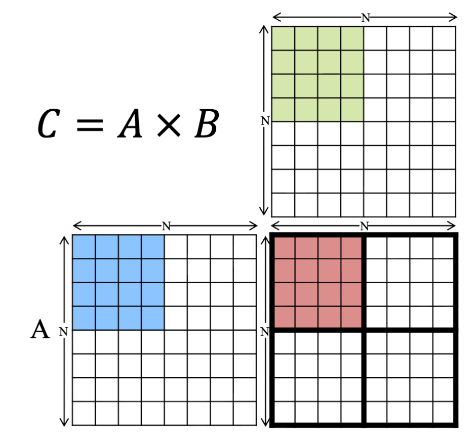 跳过 Tiling for Matrix Multiplication 的内容,我们不难发现,其实在这种算法中,对于一个元素,其实会访问 N/T 次(相比而言,naïve 方法会访问 N 次),也就是说它其实只是把 block 间的冗余去掉了,但是跨 block 的冗余还在,所以其实很容易就得出,这种情况下我们的 CGMA 就是 0.25T FLOPS/B。
想要 CGMA 变大,自然我们就是把 T 变大就好了…吗?
其实这里受限于多个因素。首先,我们是以一个 block 为单位来做 tiling 的,因此,shared memory 大小显然限制,需要满足
其次,每个 block 的线程数量是有限的,但是一个 tile 的每一个地方都应该有一个线程去访问,所以还需要满足。
其次,假设我们内存够大,线程数量够多,但也要记得我们的 SM。假设我们让 T=N,似乎一个元素就只会访存 1 次,这是最理想的情况。但在这种情况下其实我们也就只有一个 SM 在跑,其他全在闲置,算力就亏麻了。
在这种情况下,对于课程里的 Tiling,其实我们能推出一个比较好的解。
不难发现,选 32 就是最好的。当然,其实在这种情况下,我们可以算出 CGMA 是 8,仍然小于平衡点 10,所以意味着这还是一个 memory-bound 的算子,但已经比之前 0.25 好太多了。
HW1
bank conflict 啥的等 HW1 的时候再说吧,有一些什么 padding 之类的东西。我们只需要知道 即可。
P1 - MapKernel
Apply a unary function to each element of the input array and store the result in the output array 的一类算子,显然没有什么数据间的依赖,直接并行即可。
不过在这里其实就得建立一个 concept,就是 index <-> position 的转换。
具体而言,index 是指坐标的位置,例如一个 arr[3][5][10],那么我们的 index[] 就是 [3, 5, 10];而 position 是指物理上的位置,也就是说我们把一个 arr flatten 之后的实际 index,例如一个 shape[3, 5] 的数组,对于 index[1, 4],实际上 。当然,除此之外其实还有 stride 的东西,用于处理转置之类的形状,不再赘述,相信读者建立这个概念很简单。
对于 broadcast 来说,其实也就是一个把低维的和高维对齐的一个操作。举个简化的例子:
A = [[10]     [20]]
B = [[1, 2, 3]     [4, 5, 6]]

A + B = [[1 + 10, 2 + 10, 3 + 10],         [4 + 20, 5 + 20, 6 + 20]]
不难发现,其实这就是把 A 这个 shape[2, 1] 的张量拉到了 shape[2, 3],懂内存管理的小朋友肯定知道,既然我们已经有 index 数组,我们来改这个索引数组就好了,不用去对值做复制,爽死啦。
那么譬如对一个 tid = 1 (也就是指向 B 中 2 的线程),它的 indexA 数组其实就是 [0, 0],指向了 10;对于 tid = 5(指向 B 中的 6),它的 indexA 数组就是 [1, 0]。
根据这个,你大概就懂 broadcast 的实现原理了。对于小维度中的每一维度,如果它的 shape[i] > 1,那么这一维就等于 大维度中,与这一维度右对齐的分量,否则就置为 0。
这是啥意思呢,我们再换一个例子就懂了。
A = [10, 20, 30]B = [[1, 2, 3] [4, 5, 6]]现在,A 的形状是 shape[3],B 的形状是 shape[2, 3],A 比 B 少一维。对于 tid=1 来说,我们应该它与 A 中第二个数相加,也就是 indexA[1] 和 indexB[0, 1] 对应;对于 tid=5 来说,我们应该让它与 A 中第三个数相加,也就是 indexA[2] 和 indexB[1, 2] 对应。不难发现,在这种规则下,其实我们只关注它们对齐的那一维度,那么我们小的 index 也就可以从大的 index 中 infer 出来。怎么找呢?big_index[i + (num_dims_big - num_dims)] 做右对齐。
shape[2, 3]shape [3] <-- 右对齐__global__ void mapKernel( float *out, int *out_shape, int *out_strides, int out_size, float *in_storage, int *in_shape, int *in_strides, int shape_size, int fn_id){ /** * Map function. Apply a unary function to each element of the input array and store the result in the output array. * Optimization: Parallelize over the elements of the output array. * * You may find the following functions useful: * - index_to_position: converts an index to a position in a compact array * - to_index: converts a position to an index in a multidimensional array * - broadcast_index: converts an index in a smaller array to an index in a larger array * * Args: * out: compact 1D array of size out_size to write the output to * out_shape: shape of the output array * out_strides: strides of the output array * out_size: size of the output array * in_storage: compact 1D array of size in_size * in_shape: shape of the input array * in_strides: strides of the input array * shape_size: number of dimensions in the input and output arrays, assume dimensions are the same * fn_id: id of the function to apply to each element of the input array * * Returns: * None (Fills in out array) */
int out_index[MAX_DIMS]; int in_index[MAX_DIMS];
/// BEGIN HW1_1 int pos = blockIdx.x * blockDim.x + threadIdx.x; if (pos >= out_size) { return; }
to_index(pos, out_shape, out_index, shape_size);
// optional, as we have the same number of dimensions for in and out broadcast_index(out_index, out_shape, in_shape, in_index, shape_size, shape_size);
int in_pos = index_to_position(in_index, in_strides, shape_size); int out_pos = index_to_position(out_index, out_strides, shape_size);
out[out_pos] = fn(fn_id, in_storage[in_pos]); /// TODO // Hints: // 1. Compute the position in the output array that this thread will write to // 2. Convert the position to the out_index according to out_shape // 3. Broadcast the out_index to the in_index according to in_shape (optional in some cases) // 4. Calculate the position of element in in_array according to in_index and in_strides // 5. Calculate the position of element in out_array according to out_index and out_strides // 6. Apply the unary function to the input element and write the output to the out memory
// assert(false && "Not Implemented"); /// END HW1_1}P2 - ZipKernel
这里就要用到我们之前说的 broadcast 了,但是已经讲过了所以不多说了。
__global__ void zipKernel(    float *out,    int *out_shape,    int *out_strides,    int out_size,    int out_shape_size,    float *a_storage,    int *a_shape,    int *a_strides,    int a_shape_size,    float *b_storage,    int *b_shape,    int *b_strides,    int b_shape_size,    int fn_id){  /**   * Zip function. Apply a binary function to elements of the input array a & b and store the result in the output array.   * Optimization: Parallelize over the elements of the output array.   *   * You may find the following functions useful:   * - index_to_position: converts an index to a position in a compact array   * - to_index: converts a position to an index in a multidimensional array   * - broadcast_index: converts an index in a smaller array to an index in a larger array   *   * Args:   *  out: compact 1D array of size out_size to write the output to   *  out_shape: shape of the output array   *  out_strides: strides of the output array   *  out_size: size of the output array   *  out_shape_size: number of dimensions in the output array   *  a_storage: compact 1D array of size in_size   *  a_shape: shape of the input array   *  a_strides: strides of the input array   *  a_shape_size: number of dimensions in the input array   *  b_storage: compact 1D array of size in_size   *  b_shape: shape of the input array   *  b_strides: strides of the input array   *  b_shape_size: number of dimensions in the input array   *  fn_id: id of the function to apply to each element of the a & b array   *   *   * Returns:   *  None (Fills in out array)   */
  int out_index[MAX_DIMS];  int a_index[MAX_DIMS];  int b_index[MAX_DIMS];
  /// BEGIN HW1_2
  int pos = blockIdx.x * blockDim.x + threadIdx.x;  if (pos >= out_size) { return; }
  to_index(pos, out_shape, out_index, out_shape_size);
  broadcast_index(out_index, out_shape, a_shape, a_index, out_shape_size, a_shape_size);  broadcast_index(out_index, out_shape, b_shape, b_index, out_shape_size, b_shape_size);
  int a_pos = index_to_position(a_index, a_strides, a_shape_size);  int b_pos = index_to_position(b_index, b_strides, b_shape_size);  int out_pos = index_to_position(out_index, out_strides, out_shape_size);
  out[out_pos] = fn(fn_id, a_storage[a_pos], b_storage[b_pos]);
  /// TODO  // Hints:  // 1. Compute the position in the output array that this thread will write to  // 2. Convert the position to the out_index according to out_shape  // 3. Calculate the position of element in out_array according to out_index and out_strides  // 4. Broadcast the out_index to the a_index according to a_shape  // 5. Calculate the position of element in a_array according to a_index and a_strides  // 6. Broadcast the out_index to the b_index according to b_shape  // 7.Calculate the position of element in b_array according to b_index and b_strides  // 8. Apply the binary function to the input elements in a_array & b_array and write the output to the out memory
  // assert(false && "Not Implemented");  /// END HW1_2}
不过这里还得补 cuda_kernel_ops.py
lib.tensorZip( out._tensor._storage, out._tensor._shape.astype(np.int32), out._tensor._strides.astype(np.int32), out.size, len(out.shape), a._tensor._storage, a._tensor._shape.astype(np.int32), a._tensor._strides.astype(np.int32), a.size, len(a.shape), b._tensor._storage, b._tensor._shape.astype(np.int32), b._tensor._strides.astype(np.int32), b.size, len(b.shape), fn_id, )P3 - ReduceKernel
Reduce 就是要压 shape 了,我们可以不用 output_array 层面并行,可以靠 reduction operation 来并行。
__global__ void reduceKernel(    float *out,    int *out_shape,    int *out_strides,    int out_size,    float *a_storage,    int *a_shape,    int *a_strides,    int reduce_dim,    float reduce_value,    int shape_size,    int fn_id){  /**   * Reduce function. Apply a reduce function to elements of the input array a and store the result in the output array.   * Optimization:   * Parallelize over the reduction operation. Each kernel performs one reduction.   * e.g. a = [[1, 2, 3], [4, 5, 6]], kernel0 computes reduce([1, 2, 3]), kernel1 computes reduce([4, 5, 6]).   *   * You may find the following functions useful:   * - index_to_position: converts an index to a position in a compact array   * - to_index: converts a position to an index in a multidimensional array   *   * Args:   *  out: compact 1D array of size out_size to write the output to   *  out_shape: shape of the output array   *  out_strides: strides of the output array   *  out_size: size of the output array   *  a_storage: compact 1D array of size in_size   *  a_shape: shape of the input array   *  a_strides: strides of the input array   *  reduce_dim: dimension to reduce on   *  reduce_value: initial value for the reduction   *  shape_size: number of dimensions in the input & output array, assert dimensions are the same   *  fn_id: id of the reduce function, currently only support add, multiply, and max   *   *   * Returns:   *  None (Fills in out array)   */
  // __shared__ double cache[BLOCK_DIM]; // Uncomment this line if you want to use shared memory to store partial results  int out_index[MAX_DIMS];
  /// BEGIN HW1_3  /// TODO  int pos = blockIdx.x * blockDim.x + threadIdx.x;  if (pos >= out_size) { return; }  /*  [[1, 2, 3],   [4, 5, 6]]
  shape[2, 3] <-> shape[2, 1]  */
  to_index(pos, out_shape, out_index, shape_size);
  int out_pos = index_to_position(out_index, out_strides, shape_size);
  float reduced_value = reduce_value;  for (int i = 0; i < a_shape[reduce_dim]; ++i) {    out_index[reduce_dim] = i;  // actually `a_index[reduce_dim] = i`, but we can reuse out_index since they have the same number of dimensions    int a_pos = index_to_position(out_index, a_strides, shape_size);    float a = a_storage[a_pos];    reduced_value = fn(fn_id, reduced_value, a);  }

  out[out_pos] = reduced_value;
  // 1. Define the position of the output element that this thread or this block will write to  // 2. Convert the out_pos to the out_index according to out_shape  // 3. Initialize the reduce_value to the output element  // 4. Iterate over the reduce_dim dimension of the input array to compute the reduced value  // 5. Write the reduced value to out memory
  // assert(false && "Not Implemented");  /// END HW1_3}
但是如果你计算一下,你就发现这个其实并不是最优,让我们看一下:
[+] 每个元素只访存一次
[+] 每个线程循环数相同
[-] 合并访存大部分情况可能拉了。以我们代码里的例子为例,两个相邻线程访问的是相邻的行,他们之间的物理地址间隔是 4B*3 = 12B,那么他们的间隔就是 4B*3*32=384B,效率就只有 1/3 了。
[-] 并行度拉了,一个 thread 就负责要规约的那一维的一个 slice
那怎么优化呢,首先看并行度的事情,我们考虑能不能让一个 thread 还是只关注一个元素,让一个 block 才关注一个 slice,朴素的,我们可以想到每个 thread 读自己对应的元素,然后做累加。
第 0 轮: a0 a1 a2 a3 a4 a5 a6 a7第 1 轮: └┬┘ └┬┘ └┬┘ └┬┘ 4 个线程各加一对 → 4 个部分和 s1 s2 s3 s4第 2 轮: └──┬──┘ └──┬──┘ 2 个线程 → 2 个部分和 t1 t2第 3 轮: └─────┬─────┘ 1 个线程 → 总和 total大概就是
__shared__ double cache[BLOCK_DIM];
cache[threadIdx.x] = a_storage[pos_a];__syncthreads();
for (int i = 1; i < a_shape[reduce_dim]; i<<=1) {  if (threadIdx.x % (2*i) == 0 && threadIdx.x + i < a_shape[reduce_dim])    cache[threadIdx.x] += cache[threadIdx.x + i];  __syncthreads();}
if (threadIdx.x == 0) out[out_pos] = cache[threadIdx.x];
这个和我们上一版大概能有 1.8 倍多性能提升,还是比较明显的。
[2048x262144] naive 16.01 ms (134.2 GB/s) tree<256> 8.69 ms (247.1 GB/s) 1.84x当然,聪明的你可能发现了,这个其实有问题:我们假设了 ,所以实际上还要再做额外的跨步处理;此外,在 warp 层面上,你会发现这个是每个 2i 倍数的 threadIdx.x 都会跑,当 的时候,你会发现还有 个 warp 在跑,每个都只有 1 个 lane 实际在跑,这是非常浪费的。
Problem: highly divergent warps are very inefficient, and % operator is very slow
Nvidia - Optimizing Parallel Reduction in CUDA
因此,我们可以思考是不是可以把这个逆着搓一下,尽可能让后面剩下的反而都是 idx 连续的,具体我们不再赘述。事实上,在我们刚才 2048*202144 的规模下,这两版差距几乎不可见(因为是 HBM Bound,时间几乎都花在了 load 上)。如果我们降低规模,它大概在 1.45 倍左右的加速(但其实 +40% 基本上都是因为把取余换成了乘法)。
更多的优化可以看 Nvidia 这一篇
P4 - MatMul
还引入了 batch dim,但是基本上和我们之前的 tiling 大同小异。值得注意的是在 HOST 里面把 m, p 写反了,很反直觉,所以改了。
__global__ void MatrixMultiplyKernel(    float *out,    const int *out_shape,    const int *out_strides,    float *a_storage,    const int *a_shape,    const int *a_strides,    float *b_storage,    const int *b_shape,    const int *b_strides){  /**   * Multiply two (compact) matrices into an output (also comapct) matrix. Matrix a and b are both in a batch   * format, with shape [batch_size, m, n], [batch_size, n, p].   * Requirements:   * - All data must be first moved to shared memory.   * - Only read each cell in a and b once.   * - Only write to global memory once per kernel.   * There is guarantee that a_shape[0] == b_shape[0], a_shape[2] == b_shape[1],   * and out_shape[0] == a_shape[0], out_shape[1] == a_shape[1], out_shape[2] == b_shape[2].   *   * Args:   *   out: compact 1D array of size batch_size x m x p to write the output to   *   out_shape: shape of the output array   *   out_strides: strides of the output array   *   a_storage: compact 1D array of size batch_size x m x n   *   a_shape: shape of the a array   *   a_strides: strides of the a array   *   b_storage: compact 1D array of size batch_size x n x p   *   b_shape: shape of the b array   *   b_strides: strides of the b array   *   * Returns:   *   None (Fills in out array)   */
  __shared__ float a_shared[TILE][TILE];  __shared__ float b_shared[TILE][TILE];
  // In each block, we will compute a batch of the output matrix  // All the threads in the block will work together to compute this batch  int batch = blockIdx.z;  int a_batch_stride = a_shape[0] > 1 ? a_strides[0] : 0;  int b_batch_stride = b_shape[0] > 1 ? b_strides[0] : 0;
  /// BEGIN HW1_4
  // for a [m, n] and b [n, p], the output is [m, p], and for each element, we'll do n multiplications  // which needs n/TILE iterations of loading a tile of a and b into shared memory, and then computing the output tile.
  int row = blockIdx.y * TILE + threadIdx.y;  int col = blockIdx.x * TILE + threadIdx.x;  int out_pos = batch * out_strides[0] + row * out_strides[1] + col * out_strides[2];
  bool row_in_bounds = row < out_shape[1];  bool col_in_bounds = col < out_shape[2];
  float sum = 0.0f;  for (int t = 0; t < (a_shape[2] + TILE - 1) / TILE; t++) {    int a_pos = batch * a_batch_stride + row * a_strides[1] + t * TILE * a_strides[2] + threadIdx.x;    int b_pos = batch * b_batch_stride + t * TILE * b_strides[1] + threadIdx.y + col * b_strides[2];    int N = min(TILE, a_shape[2] - t * TILE);
    a_shared[threadIdx.y][threadIdx.x] = (row_in_bounds && threadIdx.x < N) ? a_storage[a_pos] : 0.0f;    b_shared[threadIdx.y][threadIdx.x] = (col_in_bounds && threadIdx.y < N) ? b_storage[b_pos] : 0.0f;    __syncthreads();
    for (int i = 0; i < N; i++) {      sum += a_shared[threadIdx.y][i] * b_shared[i][threadIdx.x];    }    __syncthreads();  }
  if (row_in_bounds && col_in_bounds) {    out[out_pos] = sum;  }  /// TODO  // Hints:  // 1. Compute the row and column of the output matrix this block will compute  // 2. Compute the position in the output array that this thread will write to  // 3. Iterate over tiles of the two input matrices, read the data into shared memory  // 4. Synchronize to make sure the data is available to all threads  // 5. Compute the output tile for this thread block  // 6. Synchronize to make sure all threads are done computing the output tile for (row, col)  // 7. Write the output to global memory
  // assert(false && "Not Implemented");  /// END HW1_4}